Overview of Energy Fluxes
FLUXCOM uses machine learning to merge energy flux measurements from FLUXNET eddy covariance towers with remote sensing and meteorological data to estimate net radiation, latent and sensible heat and their uncertainties. The resulting FLUXCOM database comprises 147 global gridded products in two setups: (1) 0.0833° resolution using MODIS remote sensing data (RS) and (2) 0.5° resolution using remote sensing and meteorological data (RS+METEO).
The visitors are referred to an overview of FLUXCOM energy fluxes for details.
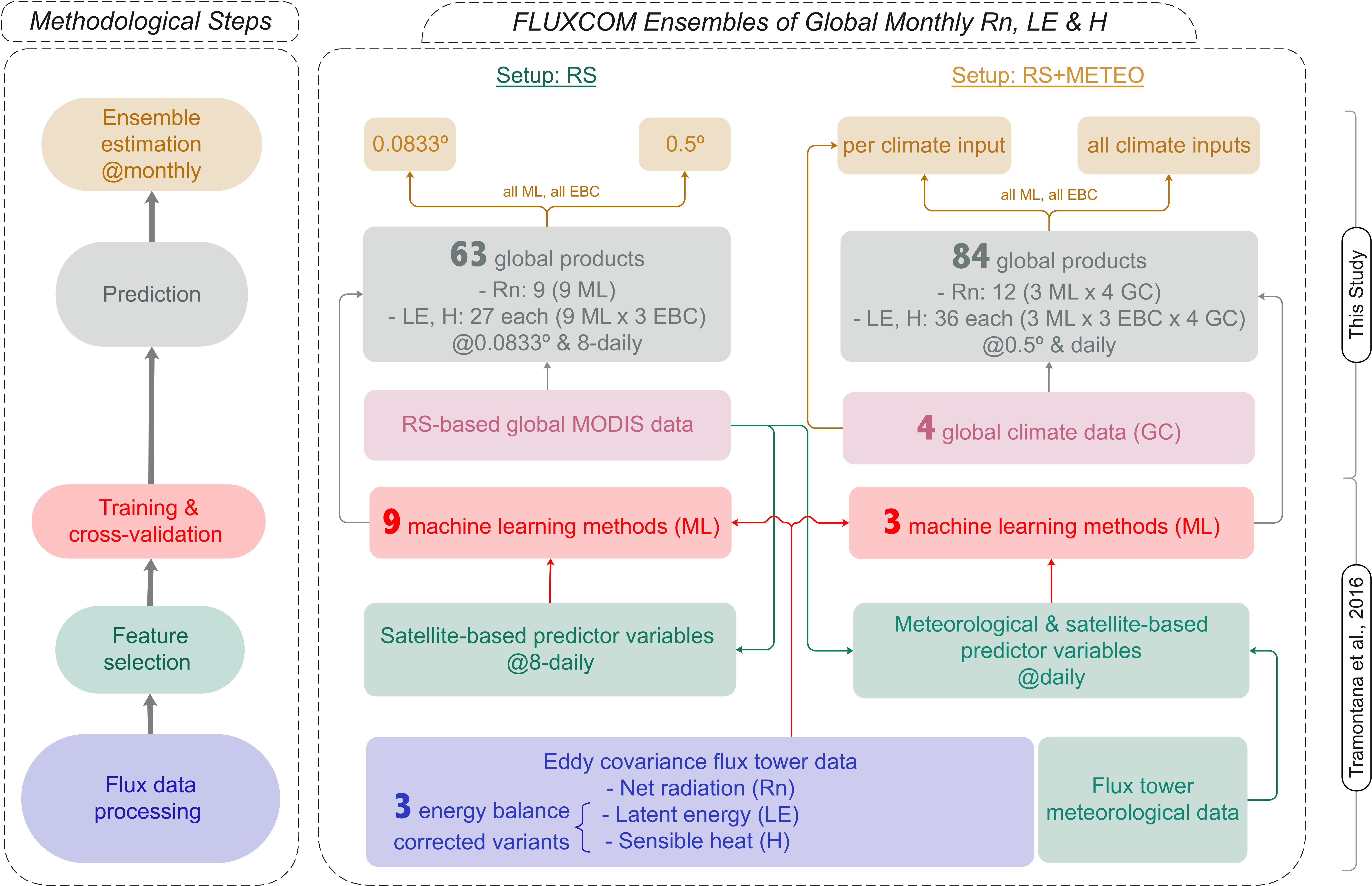
Schematic overview of the methodology and data products from the FLUXCOM initiative. The flow diagram shows the methodological steps for the remote sensing -based (RS, left) and the remote sensing and meteorological data -based (RS+METEO, right) FLUXCOM products. Final monthly ensemble products for Rn, LE, and H from RS area available at at 0.0833° and at 0.5° spatial resolution. Ensemble products from RS+METEO are available per climate forcing data set as well as a pooled ensemble. All ensemble products encompass ensemble members of different machine learning methods (ML, 9 for RS, 3 for RS+METEO) and energy balance corrections (EBC, 3 for LE and H).
Setup for Upscaling Energy Fluxes
FLUXCOM provides energy fluxes from two complementary experimental setups with respect to the input drivers (covariates) and resulting global gridded products. In the remote sensing (“RS”) setup, fluxes are estimated exclusively from Moderate Resolution Imaging Spectroradiometer (MODIS) satellite data. The second approach also exploits meteorological information. In this “RS+METEO” setup, fluxes are estimated from meteorological data and mean seasonal cycles of satellite data.
| RS | RS+METEO | |
|---|---|---|
| Product specifications | ||
| Spatial resolution | 0.0833° | 0.5° |
| Temporal resolution | 8 daily | daily |
| Time period | 2001-2015 | Depending on climate forcing |
| Climate input | n.a. | CRUNCEPv8, WFDEI, GSWP3, CERES-GPCP |
| Tiling by PFT | no | yes |
| Spatial & Seasonal patterns | f(RS) | f(RS,METEO) |
| Interannual & trend patterns | f(RS) | f(METEO) |
| Training specifications | ||
| Machine learning methods | 9: RF, ANN, MARS, MTE (3 variants), KRR, SVR | 3: RF, ANN, MARS |
| Number of flux observations for training | ~20,000 | ~200,000 |
| Spatial features | PFT, Max of MSC(fAPAR*Rg), Min of MSC(Rg) | PFT, Max of MSC(WAIU), Mean of MSC(BAND 6), Max of MSC(fPAR*Rg) |
| Spatial, seasonal features | Rpot, MSC(EVI*LSTDay) | Rpot, MSC(NDWI), MSC(LSTNight), MSC(EVI*Rg) |
| Spatial, seasonal, interannual features | Rg, LSTDay, Anom of LSTNight, Anom of (EVI*LSTDay) | Rg, Rain, Rh, RgIWAMSC(NDVI) |
The table above summarizes specifications of the FLUXCOM RS and RS+METEO setups for energy fluxes. List of acronyms: Enhanced Vegetation Index (EVI), fraction of Absorbed Photosynthetically Active Radiation (fAPAR), Leaf Area Index (LAI), daytime Land Surface Temperature (LSTDay) and night time Land Surface Temperature (LSTNight), Middle Infrared Reflectance (band 7) (MIR(1)), Normalized Difference Vegetation Index (NDVI), Normalized Difference Water Index (NDWI), Plant Functional Type (PFT), incoming global Radiation (Rg), top of atmosphere potential Radiation (Rpot), Index of Water Availability (IWA), Relative humidity (Rh), upper Water Availability Index WAI (WAIU) (for details see Tramontana et al. (2016) supplementary material, Sect. S3), Mean Seasonal Cycle (MSC) . Random forest (RF), Artificial Neural Network (ANN), Multivariate Adaptive Regression Splines (MARS), Model-Tree Ensemble (MTE), Kernel Ridge Regression (KRR), and Support Vector Regression (SVR).
Cross Validation of Energy Fluxes
Please see Tramontana et al. (2016) for details and a thorough discussion!
Different ML approaches were applied to RS and RS+METEO setups using the same sets of predictor variables, and a thorough 10-fold ‘leave-towers-out’ cross-validation was conducted. Due to the computational expense of the RS+METEO setup, only one method representing each “family” – RF, MARS, ANN and KRR – was trained.
capturing variations the across-sites, seasonal and the deviations from the mean seasonal cycle variability
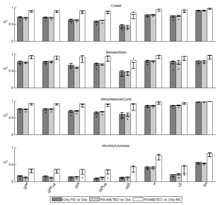
Coefficients of determination (R2) from the comparison of overall time series across-sites, mean seasonal cycle, and the anomalies, in particular: the determination coefficients between predictions by the ensemble median estimate of RS setup and observation (dark grey bars), between predictions by the ensemble median estimate of RS+METEO setup and observation (light grey bars), and between the two ensembles median estimate (white bars). Whiskers were the higher and lower R2 when the comparisons were made among the singular ML. The comparison of output by the multiple regressions was also shown (black points)
- General performance: Rn > H > LE > GPP > TER > NEE.
- Striking consistency between RS and RS+METEO.
- Between-sites variability was in general well captured by machine learning methods (best for GPP and TER). It suggests that machine learning methods are suitable to reproduce the spatial pattern of mean annual fluxes.
- Less predictive capability of the anomalies.
Global patterns of Energy Fluxes
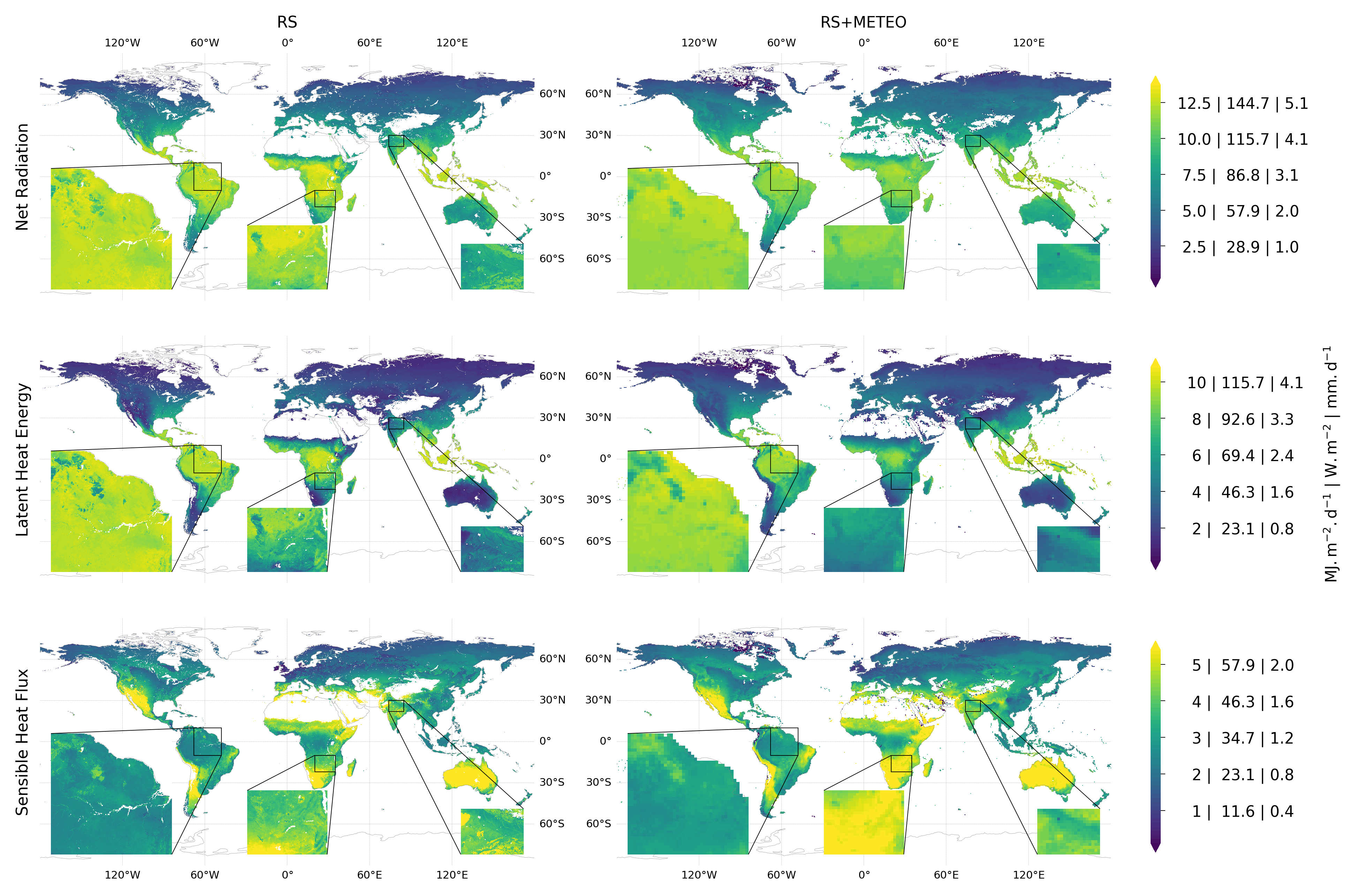
Global distributions of mean annual (2001-2013) energy fluxes from the FLUXCOM RS and RS+METEO ensembles. The first, second, and third row show net radiation, latent heat, and sensible heat fluxes, respectively (left: RS, right: RS+METEO).
Consistent with current understanding, mean annual latent heat and net radiation fluxes are the highest in tropical and the lowest in high latitude regions of the world (Figure 2). In contrast, mean annual sensible heat peaks in dry sub-tropical regions where latent heat fluxes are reduced due to expected water limitation on evapotranspiration which is known to increase the Bowen ratio (H/LE). These patterns are qualitatively consistent among the RS and RS+METEO ensemble products, while flux magnitude differences, e.g. larger net radiation of the RS product in the tropics, are also evident. In general, both RS and RS+METEO products show similar large-scale variations in energy fluxes but local-scale heterogeneities are better resolved in RS products (see the inset zoom-ins in Figure 2) due to a 6-fold increase in spatial resolution.
Global Energy Partitioning
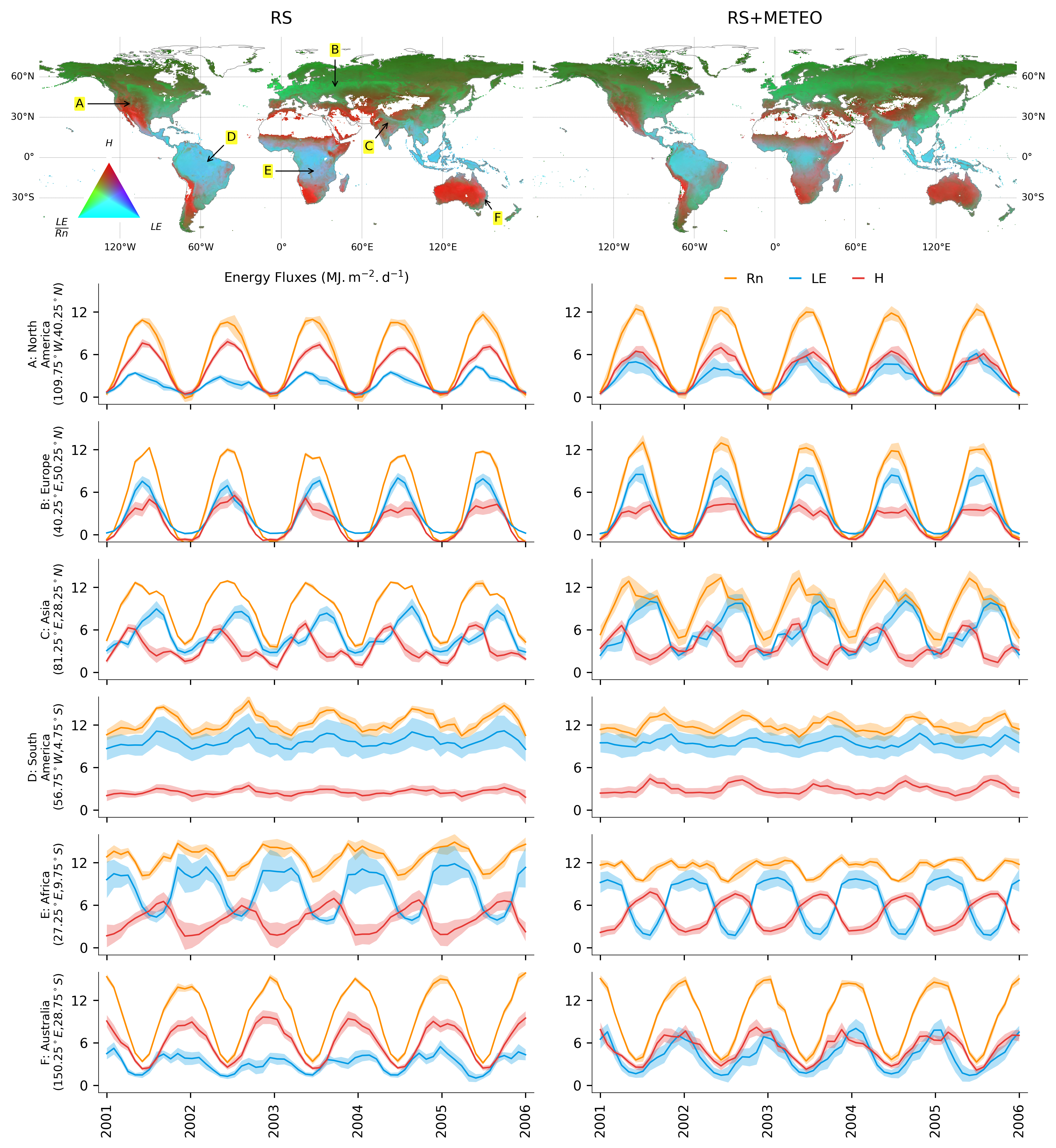
Global covariations of land-atmosphere energy fluxes, and their temporal variations and uncertainties in selected locations. RGB composite maps are with latent heat (LE) in the blue, sensible heat flux (H) in the red, and evaporative fraction (LE/Rn) in the green channel. Line plots show time series of LE (blue), H (red), and Rn (orange) for selected locations (0.5° grid cells, see map for RS) from 2001 to 2005 in MJ m-2 d-1. The shades around the lines indicate the uncertainty ranges (± 1 robust standard deviation) of ensemble members.
In these RGB maps, hot and dry regions appear as red where latent heat is low and net radiation is preferentially converted to sensible heat. Wet tropical regions with high net radiation and latent heat but low sensible heat appear as cyan. Regions where latent heat is energy limited but net radiation is intermediate or low appear in green. The partitioning of Rn into LE and H components is similar for both RS+METEO and RS products (Figure 3) with some regional differences visible. To illustrate local differences among the RS and RS+METEO ensemble products, as well as seasonal variations of energy fluxes and its uncertainties, we present time series of selected locations (0.5° grid cells) in subpanels of Figure 3. For example, in the selected location in North America (A), situated at the transition between water limited and energy limited regime of evapotranspiration, we see more H relative to LE in the RS ensemble compared to the RS+METEO ensemble. Similar patterns of slightly different net radiation partitioning in LE and H are also evident in other transitional locations in Africa (E) and Australia (F). Energy flux uncertainties (see shading in Figure 3) vary spatially, seasonally, and interannually as well as between the RS and the RS+METEO ensemble products. Where uncertainties of the RS+METEO ensemble are larger compared to the RS ensemble suggests larger contributions of meteorological forcing data uncertainty, while larger uncertainty of the RS ensemble may indicate larger contribution of machine learning method choice, perhaps due to poor constraints by flux tower stations. Overall, there is high level of consistency between the RS and RS+METEO ensemble products for seasonality and flux magnitudes as well as their uncertainties.