Two complementary strategies
Global land surface remote sensing by MODIS provides predictor variables at a high spatial resolution (e.g. 1km), but at a coarser temporal resolution (e.g. 8-daily) and only for the lifetime of MODIS (2000-present). Meteorological conditions likely provide additional information on the variability of carbon and energy fluxes that are not captured by remotely sensed surface properties alone. Utilizing meteorological predictor variables measured at FLUXNET sites requires gridded meteorological data products to produce the global flux products. Those are available for a longer time period at a finer temporal resolution (sub-daily to daily), but usually at a coarser spatial resolution (0.5° to 1°). Because gridded meteorological data are uncertain, using them in the upscaling introduces additional uncertainties in global flux products.
Therefore, FLUXCOM designed two complementary strategies:
-
Using exclusively remote sensing data at 8-daily temporal resolution (RS). This allows for generating flux products at high spatial resolution for the period after the year 2000, and without requiring uncertain gridded meteorological data.
-
Using meteorological data together with the mean seasonal cycle of the remote sensing data at daily temporal resolution (RS+METEO). This allows for generating flux products at coarse spatial but with high temporal resolution for longer time periods (e.g. since 1980). The additional uncertainty due to meteorological data sets is assessed by using several different meteorological forcing products.
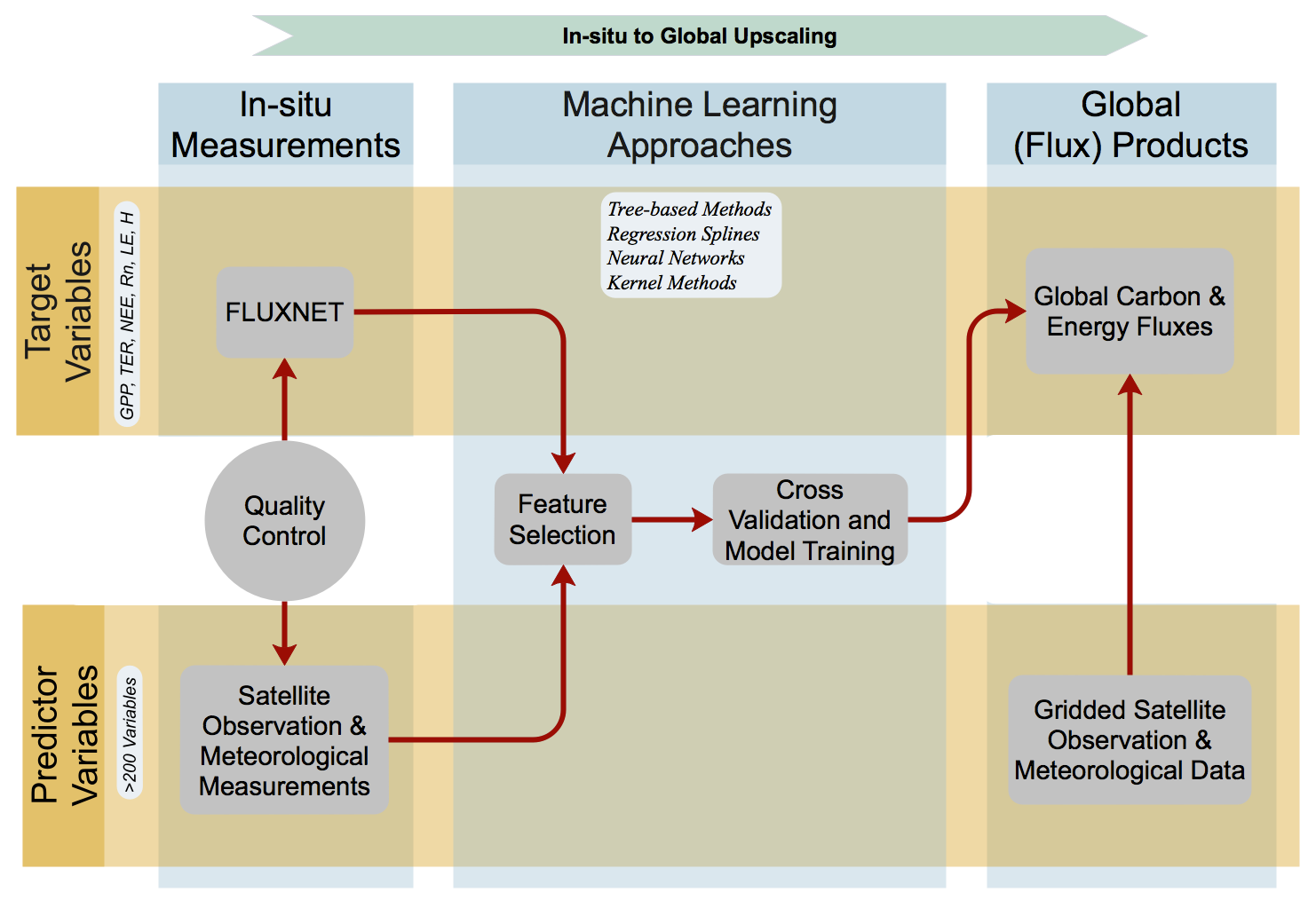
Workflow

An overview of the variables and methods used in the FLUXCOM initiative.
Machine learning algorithms
FLUXCOM uses several machine learning based regression tools that span the full range of commonly applied algorithms: from model tree ensembles, multiple adaptive regression splines, artificial neural networks, to kernel methods, with several representatives of each family. In total, FLUXCOM uses upto 11 algorithms from four broad families, which are explained briefly below:
Tree based methods
The tree based methods construct hierarchical binary decision trees. The inner nodes of the tree hold decision rules according to explanatory variables (e.g. less/greater than X1), recursively splitting the data into sub-spaces. The leaf nodes at the end of the decision tree contain models for the response variable. Because a single tree is generally not effective enough to cope with strong non-linear multivariate relationships, FLUXCOM applies two different tree ensemble methods: Random Forests (RF) that combines regression trees grown from different bootstrap samples and randomly selected features at each split node (Breiman, 2001; Ho, 1998); and Model Tree Ensembles (MTE) that combine model trees (Jung et al., 2009). FLUXCOM uses three different variants of MTE, which differ mainly with respect to different cost functions for determining the splits, and the technique to create the ensemble of model trees.
Regression splines
Multivariate regression splines (MARS) are an extension of simple linear regression adapted to non-linear response surfaces using piecewise (local) functions. The target variable is predicted as the sum of regression splines and a constant value (Alonso Fernández, 2013; Friedman et al., 1991).
Neural networks
Neural networks are based on nonlinear and nonparametric regressions. Their base unit is a neuron, where nonlinear regression functions are applied. The neurons are interconnected and organized in layers. The output of m neurons in the current layer are the inputs for n neurons of the next layer. FLUXCOM uses two types of neural networks: the artificial neural network (ANN) and the group method of data handling (GMDH). In an ANN, each neuron performs a linear regression followed by a non-linear function. The neurons of different layers are interconnected by weights that are adjusted during the training (Haykin et al., 1999; Papale et al., 2003). The GMDH is a self-organizing inductive method (Ungaro et al., 2005) building polynomials of polynomials; the neurons are pairwise connected through a quadratic polynomial to produce new neurons in the next layer (Shirmohammadi et al., 2015).
Kernel methods
Kernel methods (Shawe-Taylor and Cristianini, 2004; Camps-Valls and Bruzzone, 2009) owe their name to the use of kernel functions, which measure similarities between input data examples. FLUXCOM uses three different kernel methods: support vector regression (SVR) (Vapniket al., 1997), kernel ridge regression (KRR) (Shawe-Taylor and Cristianini, 2004), and Gaussian process regression (GPR) (Rasmussen, 2006). The SVR defines a linear prediction model over mapped samples to a much higher dimensional space, which is non-linearly related to the original input (Yang et al., 2007). The KRR is considered as the kernel version of the regularized least squares linear regression (Shawe-Taylor and Cristianini, 2004). The GPR is a probabilistic approximation to nonparametric kernel-based regression, and both a predictive mean (point-wise estimates) and predictive variance (error bars for the predictions) can be derived. In addition, FLUXCOM also uses a hybrid approach to combine RF with simple decision stumps in the inner nodes and GPR for prediction in the leaf nodes (Fröhlich et al., 2012).