Overview of Carbon Fluxes
FLUXCOM uses machine learning to merge carbon flux measurements from FLUXNET eddy covariance towers with remote sensing and meteorological data to estimate net ecosystem exchange, gross primary productivity, and terrestrial ecosystem respiration and their uncertainties. The resulting FLUXCOM database comprises 120 global gridded products in two setups: (1) 0.0833° resolution using MODIS remote sensing data (RS) and (2) 0.5° resolution using remote sensing and meteorological data (RS+METEO).
For details, refer to a comprehensive overview and synthesis of FLUXCOM carbon fluxes.
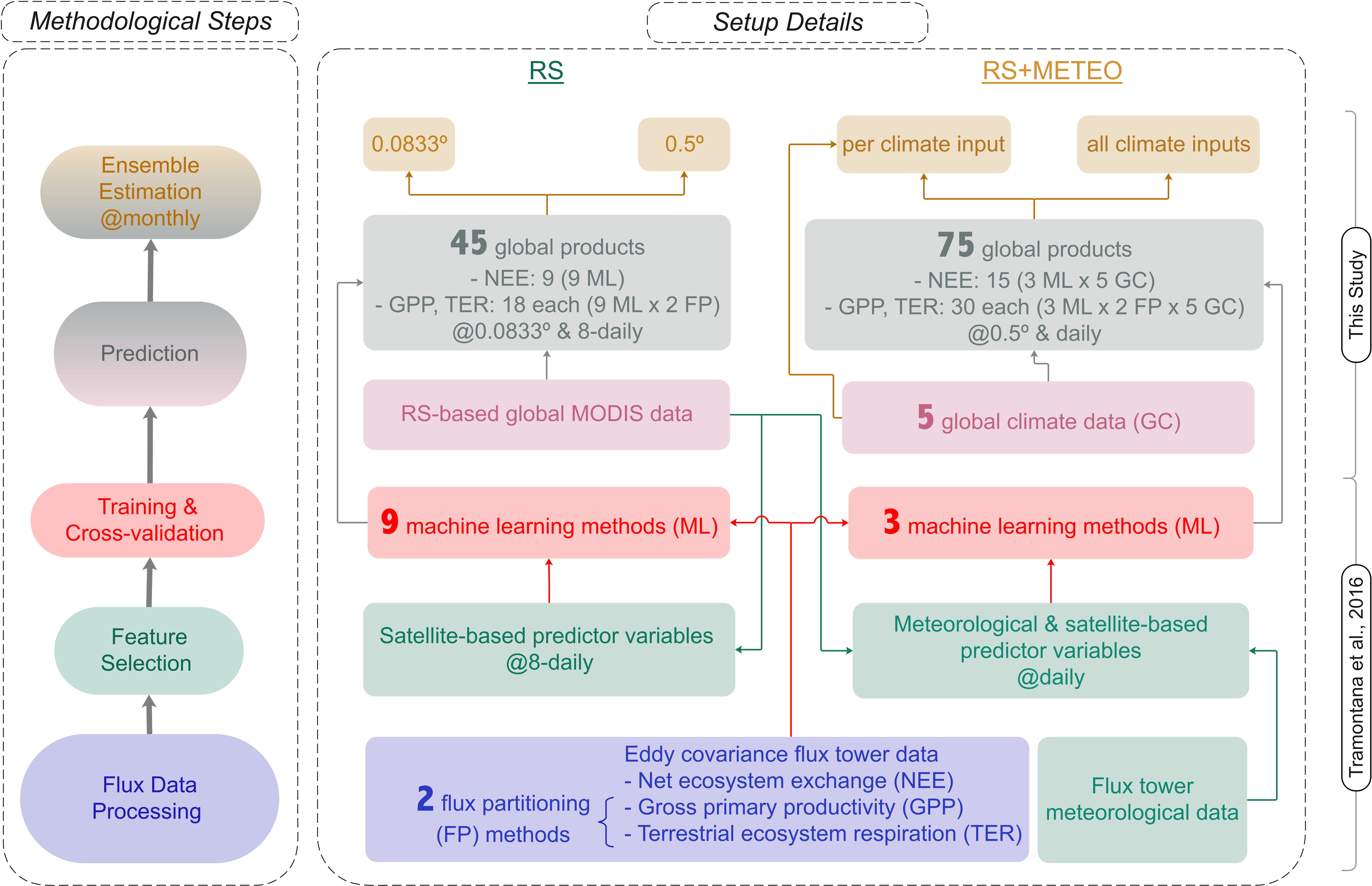
Schematic overview of the methodology and data products from the FLUXCOM initiative. The flow diagram shows the methodological steps for the remote sensing -based (RS, left) and the remote sensing and meteorological data -based (RS+METEO, right) FLUXCOM products. Final monthly ensemble products for NEE, GPP, and TER from RS are available at 0.0833° and at 0.5° spatial resolution. Ensemble products from RS+METEO are available per climate forcing (GC) data set as well as a pooled ensemble at 0.5° spatial resolution. All ensemble products encompass ensemble members of different machine learning methods (ML, 9 for RS, 3 for RS+METEO) and flux partitioning methods (FP, 2 for GPP and TER).
Setup for Upscaling Carbon Fluxes
FLUXCOM provides carbon fluxes from two complementary experimental setups with respect to the input drivers (covariates) and resulting global gridded products. In the remote sensing (“RS”) setup, fluxes are estimated exclusively from Moderate Resolution Imaging Spectroradiometer (MODIS) satellite data. The second approach also exploits meteorological information. In this “RS+METEO” setup, fluxes are estimated from meteorological data and mean seasonal cycles of satellite data.
| RS | RS+METEO | |
|---|---|---|
| Product specifications | ||
| Spatial resolution | 0.0833° | 0.5° |
| Temporal resolution | 8 daily | daily |
| Time period | 2001-2015 | Depending on climate forcing |
| Climate input | n.a. | CRUJRA_v1, ERA5, WFDEI, GSWP3, CERES-GPCP |
| Tiling by PFT | no | yes |
| Spatial & Seasonal patterns | f(RS) | f(RS,METEO) |
| Interannual & trend patterns | f(RS) | f(METEO) |
| Training specifications | ||
| Machine learning methods | 9: RF, ANN, MARS, MTE (3 variants), KRR, SVR | 3: RF, ANN, MARS |
| Number of flux observations for training | ~20,000 | ~200,000 |
| Spatial features | PFT, AMP(EVI), AMP(MIR), AMP(LSTDay) | PFT, AMP(NDVI), AMP(band 4 reflectance), MIN(NDWI), AMP(WAIL) |
| Spatial, seasonal features | MSC(LAI) | MSC(LSTNight), MSC(EVIRpot), MSC(fAPARLSTDay) |
| Spatial, seasonal, interannual features | LSTDay, LSTNight, NDVI*Rg, NDWI | WAIL, Tair, MSC(NDVI)*Rg |
The table above summarizes specifications of the FLUXCOM RS and RS+METEO setups for energy fluxes. List of acronyms: Enhanced Vegetation Index (EVI), fraction of Absorbed Photosynthetically Active Radiation (fAPAR), Leaf Area Index (LAI), daytime Land Surface Temperature (LSTDay) and night time Land Surface Temperature (LSTNight), Middle Infrared Reflectance (band 7) (MIR(1)), Normalized Difference Vegetation Index (NDVI), Normalized Difference Water Index (NDWI), Plant Functional Type (PFT), incoming global Radiation (Rg), top of atmosphere potential Radiation (Rpot), Index of Water Availability (IWA), Relative humidity (Rh), upper Water Availability Index WAI (WAIU) (for details see Tramontana et al. (2016) supplementary material, Sect. S3), Mean Seasonal Cycle (MSC), amplitude of the mean seasonal cycle (AMP). Random forest (RF), Artificial Neural Network (ANN), Multivariate Adaptive Regression Splines (MARS), Model-Tree Ensemble (MTE), Kernel Ridge Regression (KRR), and Support Vector Regression (SVR).
Cross Validation of Carbon Fluxes
Please see Tramontana et al. (2016) for details and a thorough discussion!
Different ML approaches were applied to RS and RS+METEO setups using the same sets of predictor variables, and a thorough 10-fold ‘leave-towers-out’ cross-validation was conducted. Due to the computational expense of the RS+METEO setup, only one method representing each “family” – RF, MARS, ANN and KRR – was trained.
capturing variations the across-sites, seasonal and the deviations from the mean seasonal cycle variability
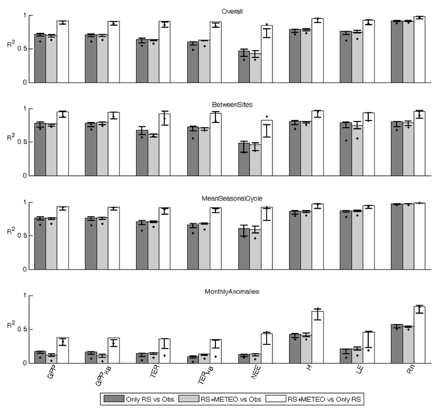
Coefficients of determination (R2) from the comparison of overall time series across-sites, mean seasonal cycle, and the anomalies, in particular: the determination coefficients between predictions by the ensemble median estimate of RS setup and observation (dark grey bars), between predictions by the ensemble median estimate of RS+METEO setup and observation (light grey bars), and between the two ensembles median estimate (white bars). Whiskers were the higher and lower R2 when the comparisons were made among the singular ML. The comparison of output by the multiple regressions was also shown (black points)
- General performance: Rn > H > LE > GPP > TER > NEE.
- Striking consistency between RS and RS+METEO.
- Between-sites variability was in general well captured by machine learning methods (best for GPP and TER). It suggests that machine learning methods are suitable to reproduce the spatial pattern of mean annual fluxes.
- Less predictive capability of the anomalies.
Evaluation of Global patterns of GPP
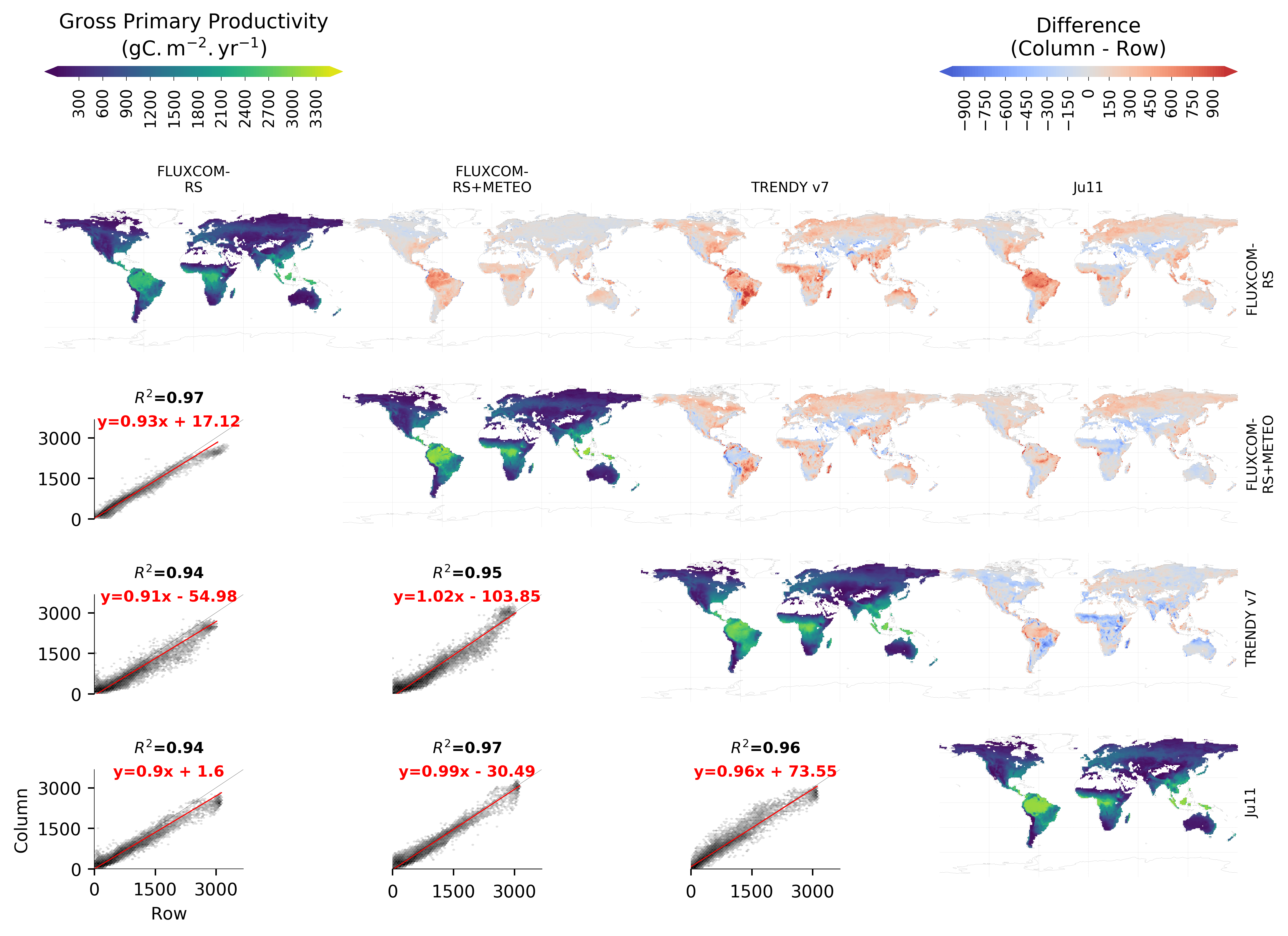
Comparisons of mean annual GPP at 1° spatial resolution for the period 2008-2010 of FLUXCOM ensemble products with Ju11 (Jung et al., 2011, MTE data) and the mean of 16 TRENDY models. Diagonal: Maps of mean annual GPP. Above diagonal: Maps of GPP differences (product along column – product along row). Below diagonal: 1:1 regression where the shading shows point density. The red line and equations show the best fit line from total least square regression..
A comparison with previous estimates of GPP indicate a high degree of cross-product (and, for FLUXCOM, also within-product) consistency of global mean GPP patterns (Figure 2). In fact, global patterns of mean GPP are consistent across both FLUXCOM ensembles (R2=0.97) as well as for Ju11 and TRENDY ensemble mean (R2>0.94), despite sizeable regional differences. The slope of the pair-wise 1:1 regressions among the different mean GPP data sets varies within ~10%. FLUXCOM-RS shows about 10-20% lower GPP than FLUXCOM-RS+METEO in the highly productive tropics and some subtropical regions. Both FLUXCOM setups estimate larger GPP than Ju11 and TRENDY in some semi-arid regions and about 5-15% lower GPP in some extratropical areas.